Monte-Carlo Consistent Partial Least Squares • plssem

The plssem package implements Monte-Carlo Consistent Partial Least Squares (MC-PLSc). This vignette gives an intuitive explanation of the core idea using a small toy example (a single correlation).

For a more formal definition see https://osf.io/preprints/psyarxiv/fwzj6_v1.

MC-PLSc starts from the observation that PLS can be a biased estimator for common factor models (e.g., models with reflective measurement), and that additional bias is introduced when ordinal indicators are treated as continuous.

The key move is to explicitly model the bias of the estimator under the assumed data-generating process, and then adjust parameters until simulated data reproduces the observed (biased) estimates.

A Toy Example: Bias From Dichotomization

Consider the correlation $r$ between continuous variables $x$ and $y$ .

set.seed(7208094)
n <- 10000
r <- 0.6
x <- rnorm(n)
y <- r * x + rnorm(n, sd = sqrt(1 - r^2))
cor(x, y)
#> [1] 0.6050904

Let’s then say that we only have access to a set of binary representations of $x$ and $y$ , $z$ and $w$ . Here we just split $x$ and $y$ in the middle.

z <- as.integer(x - mean(x) > 0)
w <- as.integer(y - mean(y) > 0)

If we calculate the correlation between $z$ and $w$ , we get a biased estimate of the underlying correlation $r$ .

cor(z, w)
#> [1] 0.4099247

Even though cor(z, w) is a biased estimate of $r$ , it is still an informative measure of $r$ . The MC-PLSc algorithm formalizes this by:

proposing a data-generating model,
simulating data under candidate parameters, and
searching for parameters that make the simulated estimator match the observed one.

In this toy example:

g() simulates binary data given a candidate value of $r$ .
f() is the estimator applied to that simulated data (here: cor()).

g <- function(r_hat, R = 5000) {
  # Generate continuous data
  x <- rnorm(R)
  y <- r_hat * x + rnorm(R, sd = sqrt(1 - r_hat^2))

  # Generate binary data
  z <- as.integer(x - mean(x) > 0)
  w <- as.integer(y - mean(y) > 0)

  # Return a data.frame
  data.frame(z, w)
}

f <- function(df) {
  # Biased correlation between binary data
  cor(df$z, df$w)
}

Putting f() and g() together, we can try different values of $\hat{r}$ and see which one reproduces the observed cor(z, w).

print(f(g(0.0)))
#> [1] 0.01282723
print(f(g(0.3)))
#> [1] 0.1791825
print(f(g(0.5)))
#> [1] 0.3203944
print(f(g(0.6)))
#> [1] 0.4191969

The true value (here, $r = 0.6$ ) gets us close, but in practice we do not know $r$ . So we rephrase this as a root-finding problem: find $\hat{r}$ such that the simulated correlation matches the observed biased one.

r_biased_observed <- cor(z, w)
h <- function(r_hat) {
  f(g(r_hat)) - r_biased_observed
}

The full MC-PLSc algorithm uses Robbins-Monro (1951) stochastic approximation, to estimate the root of $h(\hat{r})$ . Below we use a simplified approach, where we iteratively nudge $\hat{r}$ in the direction that reduces the mismatch $h(\hat{r})$ .

r_hat <- r_biased_observed # reasonable starting value
iter <- 20
history <- r_hat

for (i in seq_len(iter)) {
  temperature <- 1 / sqrt(i)
  epsilon <- h(r_hat)

  cat(sprintf("Iteration: %2d, r_hat: %.3f, epsilon: %6.3f\n", i, r_hat, epsilon))

  r_hat <- r_hat - temperature * epsilon
  history <- c(history, r_hat)
}
#> Iteration:  1, r_hat: 0.410, epsilon: -0.131
#> Iteration:  2, r_hat: 0.541, epsilon: -0.058
#> Iteration:  3, r_hat: 0.582, epsilon: -0.004
#> Iteration:  4, r_hat: 0.584, epsilon: -0.024
#> Iteration:  5, r_hat: 0.596, epsilon: -0.000
#> Iteration:  6, r_hat: 0.597, epsilon: -0.004
#> Iteration:  7, r_hat: 0.598, epsilon: -0.008
#> Iteration:  8, r_hat: 0.601, epsilon:  0.019
#> Iteration:  9, r_hat: 0.594, epsilon: -0.019
#> Iteration: 10, r_hat: 0.601, epsilon: -0.010
#> Iteration: 11, r_hat: 0.604, epsilon:  0.009
#> Iteration: 12, r_hat: 0.601, epsilon:  0.029
#> Iteration: 13, r_hat: 0.593, epsilon: -0.010
#> Iteration: 14, r_hat: 0.595, epsilon:  0.009
#> Iteration: 15, r_hat: 0.593, epsilon: -0.011
#> Iteration: 16, r_hat: 0.596, epsilon:  0.001
#> Iteration: 17, r_hat: 0.595, epsilon: -0.007
#> Iteration: 18, r_hat: 0.597, epsilon: -0.017
#> Iteration: 19, r_hat: 0.601, epsilon: -0.007
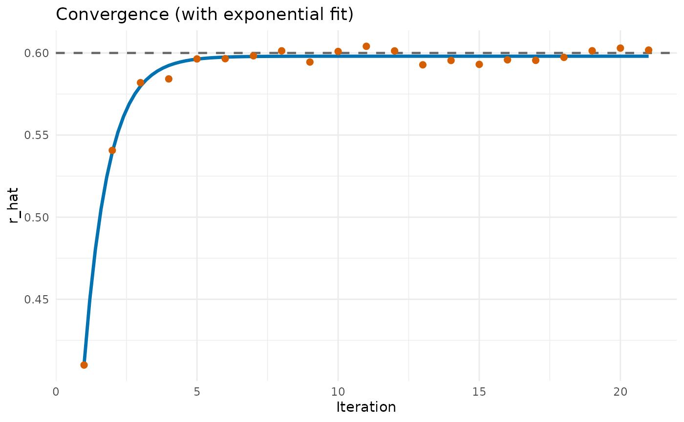
#> Iteration: 20, r_hat: 0.603, epsilon:  0.005

The sequence typically stabilizes near the underlying continuous correlation. To visualize the stabilization more clearly, we can fit a simple exponential curve to the iteration history and plot the fitted trajectory. Here we can see that we seem to approach a very good approximation of $r$ .

From The Toy Example to MC-PLSc

This toy example has the same basic structure as MC-PLSc:

g() becomes a simulator for your SEM (measurement + structural model, including the indicator scales, e.g., ordinal thresholds).
f() becomes “run PLS under the same estimation settings as for the real data, then extract the parameters of interest”.

The Monte-Carlo loop then searches for parameters that are consistent with the observed PLS estimates under the assumed data model.

Here we can see the corresponding estimates using the MC-PLSc algorithm, via the pls() function.

set.seed(2346259)
pls('y ~ x', data = data.frame(x = z, y = w),
    ordered = c("y", "x"), mcpls = TRUE)
#> plssem (0.1.2) ended normally after 26 iterations
#>   lhs op rhs   est se  z pvalue ci.lower ci.upper
#> 1   y  ~   x 0.599 NA NA     NA       NA       NA
#> 2   y ~~   y 0.642 NA NA     NA       NA       NA
#> 3   x ~~   x 1.000 NA NA     NA       NA       NA